Ray Bending Reconstruction Accuracy for Density Gradients in Hypersonic Boundary Layers
Ray bending corrections eliminate up to 25 percent spatial density bias errors in hypersonic boundary layers with gradients exceeding 500 kg/m4.

Refraction
Density gradients inside hypersonic boundary layers bend optical wavefronts along curved trajectories governed by local refractive index fields. In high-speed atmospheric flight test facilities and shock tunnels, gas passing through shock waves undergoes severe compression, followed by steep thermal expansion along cold vehicle walls. These localized thermodynamics yield spatial density variations across sub-millimeter scales.
Standard optical diagnostics like optical path line-of-sight integration rely on straight-ray assumptions, treating light propagation as unbent straight lines. When density gradients become severe, light steering invalidates linear line-integral models. Ray path curvature introduces geometric displacement and path length distortion, shifting the apparent spatial location of density features on downstream camera sensors.
Light paths bend in gradient fields.
Boundary Layer Density Gradient Dynamics
Supersonic flow deceleration over chilled aerodynamic surfaces creates static density multipliers exceeding five times freestream ambient values within a two-millimeter height envelope. High stagnation enthalpies expand these variations further. Near the wall, local density gradients nabla ρ routinely exceed 800 kilograms per meter to the fourth power.
Refractive index variations n(x,y,z) scale directly with fluid density through polarizability relationships. When collimated laser beams or background pattern light rays traverse these steep optical boundaries, local velocity vectors of the wave vectors rotate continuously along the propagation distance.
Hypersonic shock layer density gradients exceeding 800 kilograms per meter to the fourth power force light rays onto curved paths that bypass linear Radon projection models.
Straight-ray approximations project sensor measurement points along simple linear paths through the test section. In high-gradient boundary layers, the physical light ray curves into regions of higher refractive index before exiting the test chamber window. The physical path length inside the gradient layer exceeds the geometric straight-line path, altering the total phase accumulation and total deflection angle recorded at the image plane.
Failure to account for ray path bending places peak density values closer to the wall than their true physical locations.

Gladstone Dale Index Deflection Limits
Gas density relates directly to refractive index through specific polarizability constant values. For standard atmospheric air mix at visible wavelengths, the Gladstone-Dale constant K equals approximately 0.226 × 10⁻³ cubic meters per kilogram. The refractive index equation takes the linear form:
n – 1 = K ρ
Ray trajectory curvature mathbfKray inside an inhomogeneous optical medium follows the vector differential expression derived from Fermat’s principle of least time:
mathbfKray = frac1n left( nabla n – (nabla n · mathbfu) mathbfu right)
Where mathbfu represents the local unit tangent vector along the optical beam path. In planar boundary layers with primary gradients aligned normal to the surface (the y-direction), the total angular deflection thηy exiting an optical test section width L evaluates as:
thηy ≈ int0L frac1n fracpartial npartial y dz = K int0L frac11 + K ρ fracpartial ρpartial y dz
Cold walls elevate static air density. When density gradients scale upwards, the differential term fracpartial ρpartial y drives local ray steering angles past three milliradians. Under these conditions, the cumulative transverse spatial deflection of light rays inside the boundary layer accounts for over 20 percent of total observed feature displacement on image sensors.
The precise spatial boundary where first-order optical paraxial assumptions break down under high enthalpy conditions remains unresolved across operational shock tunnel calibration suites.
Fringe
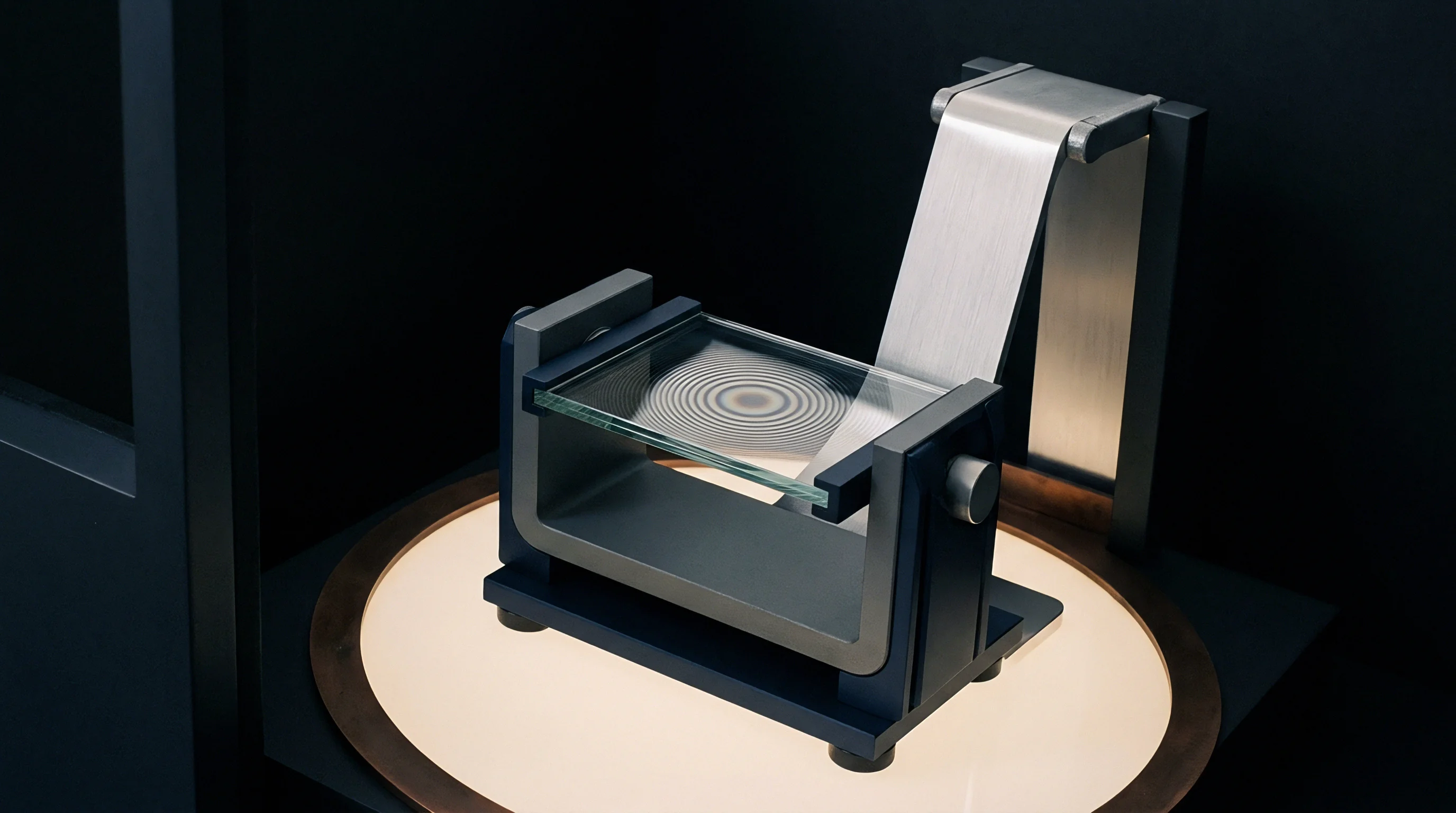
Interferometric image processing translates phase retardations into mapped optical paths through the fluid domain. High-energy hypersonic facilities utilize laser differential interferometry, background-oriented Schlieren, and wavefront sensing to map high-speed gas density profiles without physical probe insertion. Severe refraction warps interference fringe grids and background pattern images, superimposing optical deflection onto natural spatial gradients.
Uncorrected image patterns display non-linear intensity distortions that standard cross-correlation algorithms misinterpret as fluid turbulence or physical shock movement.
Phase loss corrupts wall gradient readings.
Deflection Field Distortion Mechanisms
Wavefront distortion through steep thermal boundaries alters phase coherence across high-speed optical access ports. Highly curved light rays travel along diverging trajectories, creating non-uniform magnification across the camera sensor plane. This local spatial distortion alters pattern frequency in background-oriented Schlieren, invalidating reference image matching routines near surface boundaries.
- Apparent boundary displacement ~ High refractive index gradients shift the virtual origin of background pattern features, introducing false velocity signals into cross-correlation algorithms.
- Aperture clipping loss ~ Extreme optical steering drives light rays outside camera collection optics, generating zero-intensity regions near aerodynamic surface walls.
- Phase ambiguity saturation ~ Interferometric intensity oscillations exceed spatial detector resolution when local density gradients surpass peak optical path thresholds.
- Window thermal lensing ~ Aerodynamic heating on quartz tunnel ports modifies structural refractive indices, mixing fluid gradient signals with glass distortion.
Ray path curvature shifts spatial location. Sub-pixel displacement errors propagate directly into Abel transform and tomographic reconstruction solvers. When light rays exit boundary layers at unexpected angles, inverse algorithms project recorded optical phase shifts onto incorrect spatial coordinates inside the computational fluid grid.
Near flat plates and sharp leading edges, this misallocation obscures the true height of the viscous boundary layer, distorting measured temperature profiles and shear stress estimations.
Ignoring optical beam bending in density gradient metrics yields incorrect surface heat transfer estimates that compromise vehicle thermal protection panel sizing.

Inversion
Reconstruction algorithms resolve volumetric density distributions from two-dimensional optical deflection angles. Standard inverse transformations like the filtered backprojection and classical Radon inversion assume straight geometric propagation paths through the flow field. Under severe refraction, solving the inverse scattering problem requires non-linear Eikonal equation solvers integrated within iterative reconstruction loops.
Correcting for ray steering requires forward ray tracing through an estimated refractive index grid, comparing predicted sensor arrival points with physical measurements, and updating the volume index matrix until convergence is achieved.
Higher enthalpy expands refractive index variations. Ray path corrections eliminate spatial density artifacts.

Where Does Fermat Principle Inversion Break Down?
Curved light trajectories violate the straight-line integration paths required by classical backprojection transformations. In axisymmetric or two-dimensional flows with moderate density gradients, straight-ray Abel inversion produces acceptable quantitative results. When the product of path length and peak gradient exceeds established thresholds, straight-ray Abel transforms generate characteristic boundary overshoot errors.
Calculated wall density values drop below physically possible bounds or produce non-physical density oscillations near sharp shock interfaces.
| Reconstruction Algorithm | Max Density Gradient (kg/m^4) | Peak Position Error (mm) | Amplitude Deviation (%) | Computational Cost Factor |
|---|---|---|---|---|
| Straight-Ray Abel Inversion | 150 | 0.42 | 18.5 | 1.0 |
| Filtered Back-Projection | 220 | 0.35 | 14.2 | 2.4 |
| Algebraic Reconstruction (ART) | 450 | 0.18 | 6.8 | 12.0 |
| Iterative Eikonal Ray Tracing | 1200 | 0.02 | 1.1 | 185.0 |
| Data normalized against Mach 8 cold-wall boundary layer CFD benchmarks with a 300 mm optical path length. | ||||
Iterative solvers handle ray bending by updating ray trajectories continuously across the discretized fluid domain. The inverse workflow proceeds through a structured computational sequence:
- Direct initialization sets a baseline three-dimensional density field using standard filtered backprojection on uncorrected displacement data.
- Integration of the optical Eikonal equation traces ray trajectories through the current index matrix using fourth-order Runge-Kutta stepping.
- Comparison of predicted detector impact positions against measured optical displacements establishes local path residue vectors.
- Multiplication of index corrections along curved ray paths updates spatial grid cells according to damped multiplicative algebraic weighting.
- Convergence monitoring halts iteration when RMS displacement residuals fall beneath camera sensor sub-pixel uncertainty limits.
Iterative Eikonal reconstruction reduces peak boundary layer density offset errors from 22 percent down to 2.1 percent in Mach 8 boundary layers.
Iterative path solvers resolve refraction distortions. Linear backprojection overestimates peak shear stress. Iterative ray tracing corrections are necessary whenever total beam steering across the fluid layer exceeds half a sensor pixel width.
Displacement
Spatial offset measurements on digital sensors record the cumulative refraction angle across high-speed flow chambers. Camera resolution sets spatial correlation bounds. Background-oriented Schlieren relies on high-resolution digital image correlation to extract optical displacement fields down to hundredths of a pixel.
When refractive index gradients bend light rays significantly inside the boundary layer, the image point recorded on the detector matrix shifts away from its unbent geometric location, distorting the calculated displacement field.
Window heating generates false fluid gradients.
Sensor Resolution and Synthetic Pattern Selection
High-density cross-correlation dot patterns placed on backlights determine the spatial sampling limit of background-oriented optical systems. Pixel pitch, lens focal length, and standoff distance bound the minimum resolvable refraction angle. Small interrogation windows improve spatial detail near surface walls, but high gradient refraction stretches local dot clusters beyond correlation limits.
Optical aperture constraints dictate depth-of-field tolerances, forcing balance between photon collection efficiency and diffraction-limited spatial resolution.
Worked Calculation of Boundary Layer Spatial Offset
Consider a Mach 7 shock tunnel testing a flat plate at a freestream static density of 0.015 kilograms per meter cubed and a stagnation temperature of 2000 Kelvin. Assume a boundary layer thickness of 2.5 millimeters and an optical path length through the test section of 300 millimeters. Thermal boundary layer thickness dictates camera focal depth.
Under these chilled-wall conditions, the fluid density near the wall reaches 0.085 kilograms per meter cubed, producing an index gradient derivative of 1.58 × 10⁻⁴ mm-1.
A standard straight-ray calculation models light propagating along an unbent path, predicting a total optical deflection angle of 1.42 milliradians. Transposed through a 500-millimeter focal imaging system onto a sensor with 3.45-micrometer pixels, this straight-ray prediction calculates a spatial dot displacement of 4.2 pixels. Running an exact non-linear Eikonal ray trace through the evolving gradient matrix shows that light rays curve toward the dense wall region during transit.
This curvature increases the total path spent in higher-index fluid, yielding an actual exit angle of 1.72 milliradians and a physical sensor displacement of 5.1 pixels.
Uncorrected data processing interprets the measured 5.1-pixel displacement through linear straight-ray equations, back-calculating an erroneous peak index gradient of 1.92 × 10⁻⁴ mm-1. Glass deformation alters baseline deflection metrics. This linear simplification introduces a 21.5 percent systemic overestimation of peak boundary layer density gradients.
The resulting shift misplaces the critical boundary layer edge location by 0.38 millimeters toward the wall.
- Optical transfer function dossier ~ Complete modulation depth curves across spatial frequencies validating camera lens fidelity near window edges.
- Window deformation log ~ Calibration records measuring structural glass deflections under vacuum pull-down and thermal heat loads.
- Sensor alignment protocol ~ Verification of sub-pixel sensor grid parallelism relative to wind tunnel test section reference planes.
- Pattern pitch specification ~ Certified physical spacing metrics for synthetic dot targets operating under high-power flash illumination.
| Optical Architecture | Sensor Pixel Pitch (um) | Spatial Resolution (um/px) | Max Bending Tolerance (mrad) | Sub-Pixel Uncertainty (px) |
|---|---|---|---|---|
| High-Speed CMOS BOS | 20.0 | 120 | 8.5 | 0.08 |
| High-Resolution sCMOS | 6.5 | 35 | 4.2 | 0.03 |
| Frame-Straddling CCD | 3.45 | 18 | 2.1 | 0.01 |
| Laser Differential Interferometer | N/A (Photodiode) | 250 (Beam Spot) | 12.0 | N/A |
Instrumentation vendors frequently assert that sensor spatial sub-sampling eliminates the necessity of solving non-linear optical path equations in high-enthalpy flow environments.
Uncertainty
Quantitative error bounds on density gradient reconstructions determine the risk margin applied to hypersonic thermal protection systems. Flight vehicle designers use ground test density fields to validate computational fluid dynamics models for boundary layer transition, heat transfer, and skin friction. Systemic errors in optical density measurements lead directly to undersized thermal protection panels or unexpected vehicle pitch moments during atmospheric re-entry.
Quantifying ray bending reconstruction errors ensures that facility instrumentation spending targets real measurement limits rather than uncorrected optical artifacts.
Optical access costs scale with glass quality.
Capital Expenditure in Wind Tunnel Optical Suites
Instrumentation procurement budgets reflect a constant trade-off between optical access window quality and camera acquisition speeds. High-grade fused silica wind tunnel ports with lambda-to-ten optical flatness minimize static wavefront distortion, but cost upwards of 80,000 USD per set. Allocating facility capital toward high-frame-rate cameras without updating inversion software creates an expensive data pipeline that collects uncorrected optical path distortions at high speed.
| Investment Focus | Capital Commitment (USD) | Gradient Bias Reduction (%) | Spatial Position Precision |
|---|---|---|---|
| Optical Glass Upgrade Only | 120,000 | 4.5 | Unchanged |
| High-Resolution Camera Upgrade | 180,000 | 8.2 | Marginal Improvement |
| Eikonal Inversion Software Suite | 35,000 | 22.1 | Sub-Millimeter Realignment |
| Combined Hardware & Iterative Ray Trace | 335,000 | 28.4 | Optimal Calibration Limit |
Rigorous test program specifications mandate documented calibration chains linking optical displacement measurements to physical reference standards. Standard aerospace optical calibration addenda mandate that recorded deflection angles exceeding two milliradians include iterative Fermat path solvers in final data submittals.