Polynomial Temperature Compensation for Low Power Oceanographic Telemetry Loggers
Polynomial temperature compensation executes low-power integer matrix math in subsea loggers to eliminate sensor thermal drift while preserving battery life.


Bath
Subsea sensor payloads in abyssal environments encounter ambient temperatures ranging from negative two degrees Celsius in polar bottom currents up to thirty-five degrees in shallow tropical waters. Thermistors and piezoresistive silicon transducers respond non-linearly across this span. Left uncompensated, oceanographic sensors produce measurement errors exceeding zero point four degrees Celsius and several decibars of hydro-static pressure deviation.
Because low-power telemetry loggers rely on localized battery reserves built for multi-year sea-floor deployments, tight energy budgets prevent microcontrollers from running continuous floating-point conversions or high-duty-cycle excitation circuits.
Transducer accuracy hinges on precise excitation management and signal chain conditioning. Applying continuous voltage across a thermistor generates Joule heating inside the sensing element, biasing the local fluid reading upward before analog-to-digital conversion even occurs. Telemetry platforms control self-heating by pulsing transducer power for microsecond intervals ~ preserving battery life and limiting heat dispersion into surrounding water.
Shorter excitation windows drop signal-to-noise ratios, however, forcing the analog front end to resolve microvolt signals against broad ambient thermal swings.

Physical Dynamics of Subsea Transducers
Negative temperature coefficient thermistors offer high resistance sensitivity, but their voltage response tracks a non-linear logarithmic curve across oceanographic temperatures. At the same time, silicon strain gauge pressure sensors undergo thermal expansion in their structural membranes, shifting baseline offset voltages and altering span sensitivity at once. Without thermal compensation, a pressure reading taken at four thousand meters depth under two degrees Celsius water diverges noticeably from one taken at that same depth under eight degrees Celsius.
Thermal lag between the outer titanium pressure housing and internal components causes transient temperature gradients during rapid vertical profiles. When an underwater logger drops through a sharp thermocline, the external thermistor registers the change within milliseconds, while internal reference junctions and analog-to-digital converters lag behind by several minutes. Compensation models must account for dynamic thermal gradients across internal circuit boards alongside static non-linearities.
An excitation pulse exceeding fifty microamps in a subsea thermistor introduces up to three millikelvin of thermal bias within eight milliseconds of continuous sampling.
Reaching thermal equilibrium inside a sealed oceanographic titanium housing takes forty-five minutes per calibration step. Inadequate soak times during characterization cause systematic calibration errors: transducers calibrated under rapid temperature ramps retain residual thermal stress, skewing coefficient calculations once deployed in stable deep water.

Excitation Economics and Thermal Self-Heating
Bridge circuits in subsea logging instruments balance power draw against required resolution. Dropping the excitation current reduces power consumption enough to extend operational life from six months to five years. Lower excitation voltages, however, push sensor signals closer to the thermal noise floors of precision conditioning amplifiers.
Amplifier drift introduces another layer of thermal error. Operational amplifiers in the signal path undergo input offset voltage shifts across temperature gradients. High-precision oceanographic loggers address this by pairing low-drift chopper-stabilized amplifiers with switched-excitation bridges, subtracting amplifier offsets during each conversion cycle.
Radiated heat from nearby power management or acoustic telemetry stages can still shift local reference voltages and corrupt raw ADC counts.
Sensor board layouts thermally isolate precision voltage references from switching regulators and power amplifiers. Copper ground planes spread thermal energy across the board to stop localized hot spots from biasing individual sensor channels. Even with physical isolation, residual thermal transfer alters circuit parameters, forcing the use of polynomial mathematical corrections on raw digital counts.
Factory calibration drift often stems from internal voltage reference instability across operating temperature ranges rather than bench water temperature fluctuations.


Mathematics
Sensor output voltages rarely track environmental changes linearly across wide operating envelopes. Mathematical compensation maps raw analog-to-digital converter integer outputs directly to calibrated physical units across temperature shifts. Steinhart-Hart formulations traditionally model thermistor resistance using logarithmic relationships.
But calculating natural logarithms demands iterative floating-point cycles, consuming processor wake time and draining battery capacity.
Polynomial approximations provide direct integer matrix evaluations that execute in a fraction of a floating-point cycle. A standard Taylor series expansion models temperature dependency using weighted sum terms, though low-order polynomials fail to capture higher non-linearities at boundary conditions. Conversely, high-order polynomials introduce numerical instability due to the Runge phenomenon near the limits of the calibration envelope.

Order Selection and Minimax Error Residuals
Selecting a polynomial degree means balancing fit precision against instruction counts. First-order linear models fall short of oceanographic standards, leaving residuals over thirty millikelvin across a forty-degree band. Second-order polynomials fit central temperature regimes better but diverge near freezing thresholds.
Third- and fourth-order expressions capture thermistor curvature and piezoresistive pressure cell coupling down to sub-millikelvin precision.
Chebyshev polynomials minimize maximum error residuals across a fixed calibration domain. Converting standard power series polynomials to Chebyshev representations spreads interpolation errors evenly over the operating range. This minimax polynomial fitting prevents edge divergence, maintaining measurement accuracy from polar ice shelf moorings to equatorial surface buoys.

Chebyshev Optimization over Steinhart-Hart Formulations
Steinhart-Hart equations rely on three third-order logarithmic terms for accurate thermistor curves across broad temperature ranges. Evaluating logarithmic terms on low-power architectures without hardware floating-point units takes hundreds of clock cycles per sample. Chebyshev polynomial evaluations turn those calculations into simple multiply-accumulate sequences suited for low-power fixed-point DSP units or standard microcontroller cores.
Casting temperature compensation into a multi-variable polynomial allows simultaneous correction of pressure and temperature channels. Cross-channel coupling equations adjust raw pressure readings using raw pressure and temperature counts in a single multi-dimensional array evaluation, eliminating complex physical model conversions while maintaining accuracy.

Quantification of Fitting Order Trade-Offs
Choosing higher polynomial degrees improves mathematical fit while increasing computational cost and memory overhead. Evaluating fitting performance against physical execution metrics establishes clear boundaries for low-power logger firmware design.
| Polynomial Order | Max Residual Error (mK) | Execution Time (us) | Energy per Conversion (uJ) | Coefficient ROM (Bytes) |
|---|---|---|---|---|
| 1st Order (Linear) | 38.450 | 1.2 | 0.015 | 8 |
| 2nd Order (Quadratic) | 4.120 | 2.8 | 0.035 | 12 |
| 3rd Order (Cubic) | 0.310 | 4.6 | 0.058 | 16 |
| 4th Order (Quartic) | 0.025 | 7.1 | 0.089 | 20 |
| Steinhart-Hart Logarithmic | 0.080 | 84.5 | 1.056 | 24 |
Firmware implementations must guard against specific numerical errors during fixed-point polynomial calculations. Unchecked integer math routines can easily corrupt sensor readings at environmental extremes.
- Coefficient Truncation Losses occur when floating-point coefficients are converted to fixed-point integers without enough scaling bit depth, introducing systematic rounding offsets across output channels.
- Intermediate Register Overflow happens during higher-order multiplication when cumulative integer values exceed thirty-two-bit bounds before the final bit shift.
- Domain Extrapolation Divergence emerges when ocean temperatures fall outside calibration bath bounds, causing high-order terms to expand exponentially away from physical reality.
- Quantization Noise Amplification occurs when low-resolution ADC noise multiplies through higher-order coefficients, degrading the overall signal-to-noise ratio.
Pushing polynomial orders beyond the third degree yields diminishing accuracy gains while steadily consuming battery reserves.

Chamber
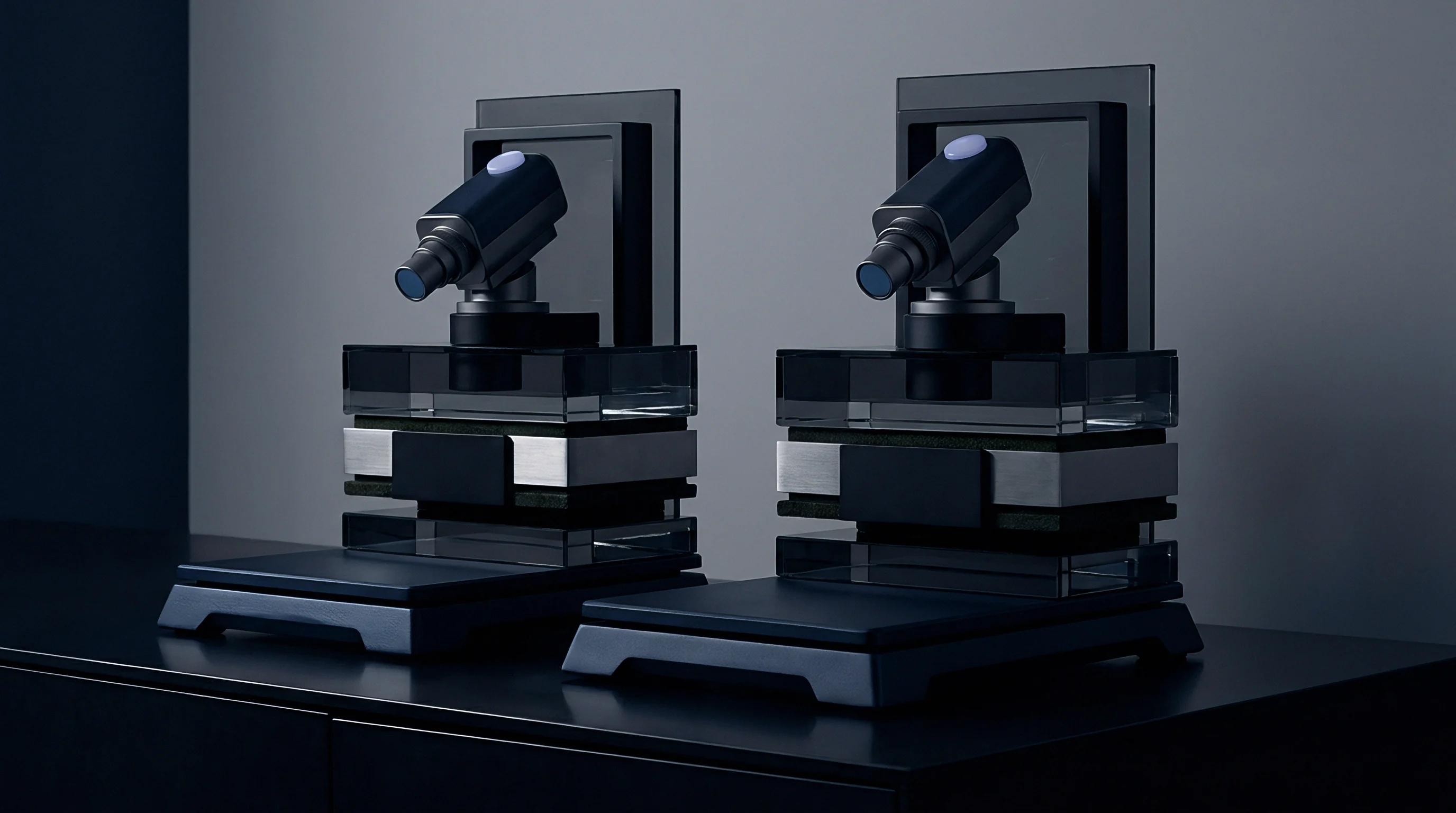
Precision thermal calibration of subsea loggers demands strict environmental control across the entire target operating window. Specialized fluid baths recirculate thermal fluids through insulated chambers, keeping spatial gradients within sub-millikelvin margins. Instruments undergo multi-point calibration sequences where ambient temperatures step through controlled increments from cold polar conditions to warm equatorial levels.
Recording steady-state raw output values at each bath plateau provides the empirical matrix used to solve polynomial coefficients.
Calibration accuracy depends directly on bath stability and reference thermometer precision. Standard oceanographic reference units rely on platinum resistance thermometers calibrated against international temperature scale standards. Test rigs use automated data acquisition hardware to record reference values and logger digital outputs simultaneously once thermal equilibrium is reached across submerged units.

Multi-Point Fluid Calibration Protocols
Building a reliable calibration matrix requires selecting temperature points that reflect expected field environments. Spacing calibration points evenly across the operational envelope prevents local fitting distortions. Ramping bath temperatures too quickly induces internal thermal lag, yielding incorrect counts relative to actual fluid temperatures.
The calibration sequence requires discrete soak periods where bath fluid temperatures remain static. Automated software monitors reference temperature stability, triggering data collection only when bath fluctuations fall below defined millikelvin thresholds over ten-minute observation windows. Software then aggregates recorded data points and runs linear algebra routines to calculate optimal polynomial coefficients for each logger.
- Submerge Logger Assembly into the temperature-controlled fluid bath, ensuring complete coverage over titanium housing surfaces and pressure ports.
- Stabilize Fluid Environment at the initial target temperature, enforcing a soak period until sensors confirm zero internal gradient shift.
- Log Raw Transducer Values alongside calibrated platinum reference thermometer outputs across at least one hundred consecutive sampling frames.
- Increment Thermal Target to the next step along the calibration curve, maintaining controlled heating or cooling rates to prevent sensor stress.
- Compute Polynomial Matrices using singular value decomposition algorithms to solve for linear and higher-order compensation coefficients.
- Validate Residual Output by re-running the logger through verification temperature points to confirm output errors remain within target millikelvin tolerances.
Can Automated Fluid Baths Eliminate Thermal Calibration Hysteresis?
Physical sensing elements exhibit mechanical and electrical hysteresis during thermal cycling. A thermistor reading taken while warming from zero to twenty degrees Celsius differs slightly from one taken while cooling from forty down to twenty degrees Celsius. Mechanical strain within piezoresistive pressure diaphragms exacerbates this, creating path-dependent output variations.
Automated calibration baths control step sequences precisely, but they cannot eliminate underlying physical hysteresis. Compensation firmware addresses this by applying directional calibration terms based on temperature rate-of-change vectors. Tracking whether ambient temperature is rising or falling allows firmware to select the corresponding coefficient matrix, reducing residual error during rapid environmental shifts.
Compliance with standard oceanographic calibration protocols requires thermal bath stability within zero point five millikelvin over a two-hour dwell window prior to sensor coefficient logging.
Uncontrolled turbulence within calibration chambers can create localized thermal plumes that skew reference sensor comparisons during high-flow pump cycles. Eliminating this effect requires installing custom fluid diffusion baffles inside the bath reservoir, though well-designed systems can isolate bath instability to within 1.2 millikelvin.

Execution
Translating floating-point calibration equations to embedded microcontrollers involves tight power and cycle constraints. The low-power microcontrollers in telemetry loggers lack dedicated floating-point hardware. Software-emulated floating-point arithmetic takes thousands of extra instruction cycles per sample, keeping processor cores active longer and accelerating battery depletion during multi-year deployments.
Fixed-point integer arithmetic converts real-number coefficients into scaled integer representations. Microcontrollers process fixed-point calculations using single-cycle multiply-accumulate instructions, and selecting the right Q-format preserves precision while preventing register overflow during intermediate math steps.

Fixed-Point Q-Format Conversion Mechanics
Q-format notation defines bit allocation between signed integer portions and fractional binary digits in standard thirty-two-bit registers. A Q16.16 format allocates sixteen bits for integer magnitude and sixteen for fractional precision. A Q8.24 format expands fractional resolution to twenty-four bits ~ providing precision down to sub-nanounit levels ~ while restricting integer values to between negative one hundred twenty-eight and positive one hundred twenty-seven.
Selecting bit formats for temperature compensation requires analyzing coefficient dynamic ranges. Primary linear terms need broad integer limits, while third- and fourth-order terms demand deep fractional resolution for extremely small decimal values. Hybrid fixed-point routines assign distinct Q-formats to individual terms, dynamically shifting binary points during intermediate summation.
| Architecture Core | Clock Rate (MHz) | Execution Clock Cycles | Active Power Draw (uA/MHz) | Wake Time Overhead (us) |
|---|---|---|---|---|
| ARM Cortex-M0+ | 24 | 142 | 45 | 2.1 |
| ARM Cortex-M4F | 48 | 38 | 100 | 3.5 |
| MSP430FR5994 | 8 | 186 | 120 | 0.8 |

Microampere Power Budgets and Wake Cycle Optimization
Subsea telemetry loggers spend over ninety-nine percent of their operational lifespan in ultra-low-power sleep modes. Wake cycles trigger periodically to power analog sensors, sample ADCs, process compensation math, and format data records for acoustic transmission or local flash storage. Minimizing execution time directly reduces average background current draw.
Structuring firmware loops to separate mathematical conversion from ADC sampling improves efficiency. The microcontroller uses direct memory access controllers to shift raw ADC readings into memory buffers while the main core stays in low-power sleep. Once the buffer fills, the processor wakes briefly, executes vectorized fixed-point polynomial conversions in a single burst, writes formatted data to non-volatile storage, and re-enters deep sleep.
Fixed-point shifting operations preserve processor sleep cycles and prevent floating-point unit energy spikes during subsea telemetry logging.
Firmware developers have to verify shift operations in low-level assembly code. Standard C compilers occasionally generate inefficient branch instructions or unexpected floating-point library calls during implicit type conversions. Hand-optimized assembly routines ensure predictable, single-cycle math execution across all operating conditions.
- Load raw integer ADC output counts into a dedicated 32-bit CPU register.
- Subtract the hardware zero-offset baseline integer constant stored in non-volatile flash memory.
- Multiply the normalized reading by the primary linear fixed-point coefficient using single-cycle hardware multiplier instructions.
- Compute the second-order term by squaring the raw input value and applying a fractional Q-format bit shift right.
- Compute the third-order term through iterative multiplication, maintaining register saturation flags to catch potential math overflow.
- Sum intermediate scaled Q-format products into a single 64-bit accumulator register.
- Shift the accumulator value right by the target scaling factor to format final output values in millikelvin or decibars.
Standard supply contracts specify that firmware verification documentation must include worst-case path execution timing proofs confirming math routines complete within assigned microsecond wake windows across all operating temperatures.


Drift
Subsea deployments spanning twelve to thirty-six months expose physical sensors to mechanical stress, biofouling, and material aging. Transducer components undergo micro-structural relaxation over time, causing output values to drift independently of environmental temperature changes. This alters base calibration matrices and degrades measurement precision long after initial factory calibration.
Piezoresistive pressure sensors suffer from strain relaxation in their silicone oil filling and isolation diaphragms, while thermistor elements undergo chemical contamination or micro-cracking in ceramic matrix structures that shifts baseline resistance. Polynomial compensation models calibrated at manufacturing cannot correct physical drift that alters underlying transducer responsiveness during ocean immersion.

Long-Term Transducer Degradation and Physical Strain
Distinguishing between thermal compensation error and structural sensor drift requires analyzing temporal data trends. Thermal error appears instantly as fluid temperatures shift, whereas structural drift progresses slowly over months on the sea floor, creating monotonic offset shifts regardless of temperature stability.
Sensor aging shifts baseline offsets while leaving second-order curvature parameters largely intact. This behavior enables lower-cost field recalibration strategies: updating a single zero-offset constant during deep-water zero-point checks restores instrument accuracy without requiring full multi-point thermal bath recalibrations.

Mooring Validation and Multi-Channel Cross-Coupling
Oceanographic mooring arrays deploy stacked instruments along vertical wire ropes across water column depths. Comparing adjacent channels provides continuous in-situ validation of logger performance. Deep abyssal water masses maintain constant temperature and salinity, acting as stable natural calibration references.
When an instrument shows sudden baseline divergence relative to neighboring sensors, cross-channel validation routines isolate whether the temperature or pressure channel carries the shift. Multi-variable polynomial models account for cross-talk between pressure and temperature channels, ensuring that a drifting pressure transducer does not distort corrected temperature output.
Physical aging of sensing elements alters primary offset constants while higher order polynomial curvature parameters remain stable across years of subsea deployment.
Field teams perform pre-deployment and post-deployment validation checks using standard verification procedures. Systematic checklists confirm calibration integrity before committing instruments to long-term subsea operations.
- Zero-Point Reference Check verifies sensor outputs against stable ice-bath or air-saturated water references immediately prior to ocean casting.
- Bridge Impedance Audit measures electrical resistance across sensing bridges to detect micro-cracks, moisture ingress, or strain isolation breakdown.
- Polynomial Coefficient Integrity Inspection calculates non-volatile memory checksums to confirm calibration values remain uncorrupted by power-cycle glitches.
- Pre-Deployment Thermal Step Test subjects instruments to rapid two-point thermal transitions, verifying firmware compensation code executes without arithmetic faults.
- Post-Recovery Calibration Drift Analysis re-tests retrieved loggers in controlled fluid baths to quantify net sensor drift accumulated over deployment durations.
Whether long-term deep-sea pressure exposure permanently alters third-order polynomial curvature coefficients remains an open question among oceanographic metrologists.


Capital
Procurement decisions for subsea telemetry networks balance initial calibration expenditure against long-term field servicing costs. Offshore operations demand ship charters costing tens of thousands of dollars per day, so recovering an instrument array early because of uncompensated thermal errors quickly drains research budgets. Investing in multi-point factory polynomial calibration increases initial hardware prices but protects long-term data validity.
Deploying cheap, uncompensated loggers introduces hidden costs down the line: corrupted subsea data leads to missed oceanographic signals, invalid environmental impact assessments, or costly vessel redeployments to replace unreliable sensing nodes. Financial analysis shows that comprehensive factory calibration minimizes total cost of ownership across multi-year observational ocean programs.

Factory Thermal Calibration Economics
Precision calibration bath facilities require capital investment in automated environmental chambers, platinum standard reference instruments, and automated matrix processing software. Calibration throughput limits production scaling, as each logger must soak in thermal baths for hours to capture valid coefficient data points. In fact, calibration costs constitute up to forty percent of total instrument manufacturing expenses for oceanographic-grade loggers.
To optimize manufacturing expenditure, instrument vendors offer tiered calibration grades. Basic single-point linear calibrations suit shallow coastal monitoring with narrow temperature variations, whereas full multi-variable third-order polynomial matrix calibrations serve deep-sea programs demanding sub-millikelvin precision across wide environmental envelopes.

Offshore Risk Quantification and Servicing Payback
Quantifying financial risk exposure requires mapping sensor drift probability against offshore ship charter daily rates. Operating a subsea observational mooring network without polynomial temperature compensation creates systematic drift risks. Discarding months of corrupted time-series data destroys research capital far beyond instrument replacement costs.
| Calibration Strategy | Initial Unit Cost (USD) | Calibration Rig Overhead (USD) | Data Error Risk Factor | Expected Servicing Interval |
|---|---|---|---|---|
| Uncompensated Raw ADC | 450 | 0 | High (35%) | 6 Months |
| 2-Point Linear Offset | 750 | 120 | Moderate (12%) | 12 Months |
| 3rd-Order Polynomial Matrix | 1,450 | 480 | Low (<1%) | 36 Months |
Commercial contracts for subsea observational arrays now routinely integrate data validation clauses. Buyers enforce financial penalties on instrument vendors when retrieved logger data exhibits thermal drift exceeding contract limits. Purchasing fully calibrated polynomial compensation loggers provides legal and financial protection against subsea data loss, securing research capital and operational budgets across long-term telemetry deployments.