Standard Temperature Correction Integration within Automated ERP Inventory Valuation
Standard temperature correction converts ambient bulk liquid receipts into standard volume, eliminating phantom inventory and securing balance sheet accuracy.


Tank
Terminal meters record gross observed volume at whatever temperature the custody transfer line maintains during discharge. Liquid hydrocarbons, bulk petrochemicals, and ethanol shrink when cooled and expand when heated, changing the volume a given mass occupies without altering the mass delivered. If an automated ERP system posts an uncorrected receipt of four hundred thousand barrels discharged at ninety-five degrees Fahrenheit, it books an ambient volume that drops to three hundred ninety-three thousand barrels once the fluid cools to sixty degrees in storage.
That leaves seven thousand phantom barrels on the balance sheet. Uncorrected receipts like this dilute unit costs, distort standard calculations, and leave finance teams chasing unexplained inventory losses during physical audits.
Hydrocarbon accounting handles this behavior through standard temperature correction. Converting gross observed volume to gross standard volume at a fixed base temperature gives a stable, mass-equivalent baseline across procurement and inventory cycles. In North America and regions aligned with API measurement standards, sixty degrees Fahrenheit is the standard benchmark.
Europe, Asia, and jurisdictions tied to international metrological frameworks rely on fifteen degrees Celsius or twenty degrees Celsius. Automated valuation engines use standard volume to value inventory ledgers, reserving gross observed volume for tank capacity checks and logistics planning.
Custody contracts executed under API MPMS Chapter 11.1 establish gross standard volume at sixty degrees Fahrenheit as the sole basis for invoice settlement.
When enterprise systems process bulk liquid movements, they pull data directly from tank gauging systems, SCADA networks, and electronic flow computers. Meters with resistance temperature detectors sample the fluid stream hundreds of times a minute, passing gross volume, observed temperature, line pressure, and measured density into staging tables within the ERP software. From there, the valuation module applies volume correction factors from standard industry algorithms to calculate net fiscal volume before posting the material document to the general ledger.

Automated Hydrocarbon Valuation Architecture
Valuation discrepancies emerge whenever enterprise software treats bulk liquids like discrete inventory. A pallet of valves holds its count whether a warehouse is freezing or ninety degrees. A tank of heavy fuel oil, by contrast, fluctuates constantly in liquid height even though the total mass hasn’t changed.
ERP platforms without native temperature-correction logic treat liquid movements as simple volumetric math, creating artificial gains during warm summer receipts and artificial write-downs in winter.
Fixing this requires decoupling financial valuation quantities from physical storage volumes. Modern ERP platforms manage that separation through secondary quantity management modules, tracking multiple units of measure simultaneously in the material master record: ambient volume for operational tank capacity, gross standard volume for inventory valuation, and metric mass for statutory and customs filings. The system then uses gross standard volume to update moving average prices, value standard cost inventory, and clear GR/IR accounts against incoming supplier invoices.
Field measurements and financial postings also need tight synchronization. If an automated system takes in liquid at eighty degrees Fahrenheit and calculates standard volume using a static, outdated density value, the inventory balance inherits a pricing error that propagates through the bill of materials into finished product costs. Manufacturing units consuming that liquid as feedstock then display false usage variances, mistaking volumetric measurement drift for actual yield loss.

Custody Transfer Interface Protocols
Automated data collection at the marine terminal, pipeline manifold, or rail rack captures raw physical parameters before any ledger entry is created. Modern electronic custody transfer units compile batch transaction records with gross observed barrels, average flowing temperature, line pressure, and base density measured by inline digital densitometers. These values pass to the enterprise middleware layer through OPC protocols or structured file transfers.
The middleware maps this raw telemetry into business transaction objects, screening incoming records for sensor faults, sudden thermal spikes, and density readings outside commercial tolerances. If a pipeline batch arrives with a failed temperature sensor, the system quarantines the record for manual review rather than posting an inaccurate gross standard volume to the financial core.
Commercial contracts demand precise calculations. A shift of one-tenth of a degree Fahrenheit on a five-hundred-thousand-barrel crude cargo changes standard volume by hundreds of barrels ~ a financial swing of tens of thousands of dollars on one receipt document. Automated enterprise valuation engines avoid manual spreadsheet calculations by executing standard temperature correction algorithms directly in the database layer, leaving a clean audit trail from receipt to balance sheet.
General commercial terms across pipeline delivery points typically specify that bill of lading quantities calculated via volume correction factors supersede shore tank readings for invoicing, binding both parties to standard volume regardless of temperature shifts during transit.
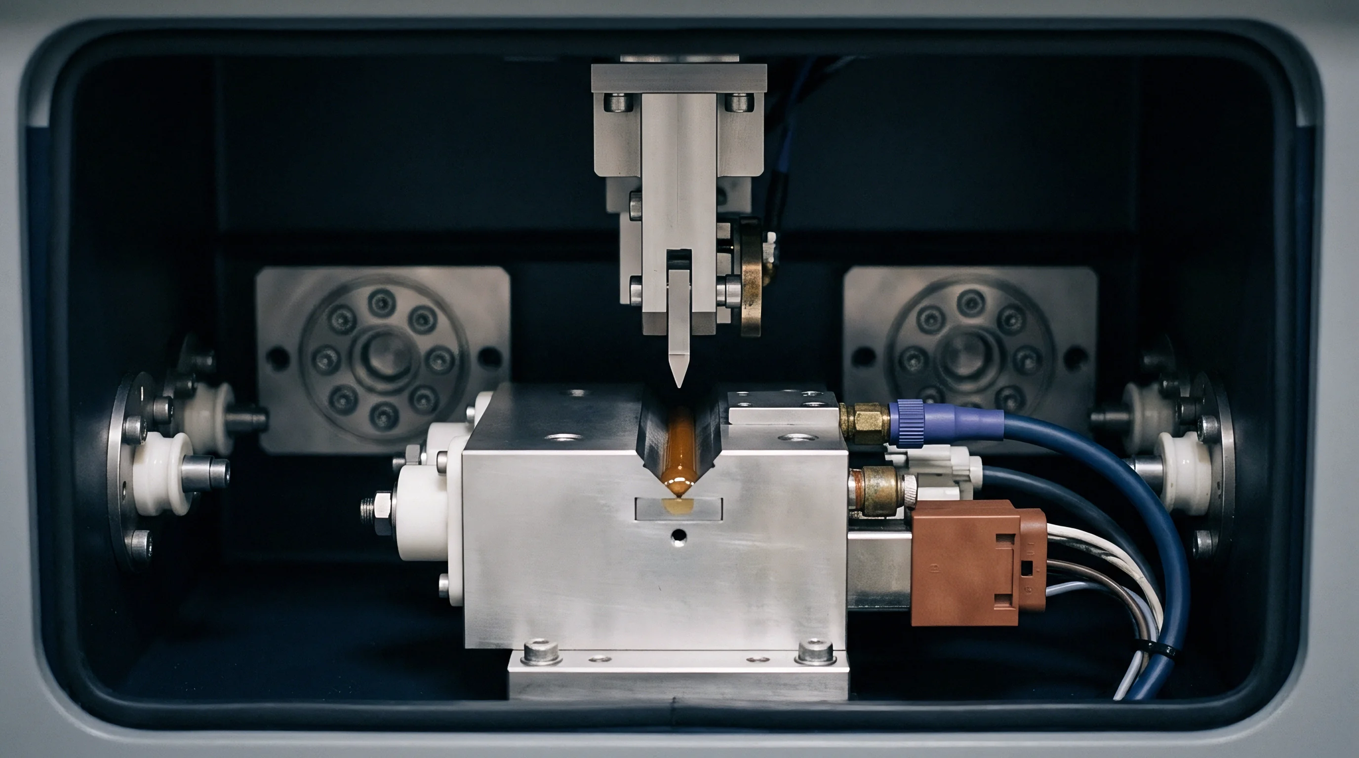

Expansion
Petroleum liquids, chemical solvents, and biofuels expand and contract far more than solid commodities. This volumetric response to temperature isn’t linear ~ it varies across fluid densities and thermal ranges. Light naphtha and LPG expand rapidly as temperatures rise, while heavy residual fuels and bitumen show much smaller volume shifts per degree.
Accounting for this thermal behavior is central to automated inventory tracking.
As ambient temperature climbs, intermolecular spacing increases, lowering fluid density while total mass stays constant. Cooling pulls molecules closer, raising density and reducing ambient volume. A tank holding light crude oil at forty degrees API gravity experiences a volume change of roughly zero point zero six percent per degree Fahrenheit.
Over a thirty-degree seasonal shift, uncorrected storage volume drifts by nearly two percent, creating tens of thousands of dollars in phantom inventory gains or losses if accounting relies on raw gauge height.
That temperature-volume relationship is defined by the thermal expansion coefficient. Because this coefficient shifts as temperatures drift from base conditions, standards organizations developed empirical equations that calculate exact volume correction factors across hydrocarbon grades. Enterprise software embeds these equations into goods receipt transactions, replacing static conversion multipliers with live calculations.

Which Base Temperature Controls the Material Valuation?
The choice of baseline reference temperature determines how the valuation engine standardizes physical volume across regional assets. Global supply chains rely on two main measurement frameworks, so ERP platforms must support multi-base conversion matrices within a single general ledger architecture.
In North America, sixty degrees Fahrenheit is the legal and commercial baseline for petroleum inventory. The valuation engine converts all field measurements ~ whether recorded at twenty degrees in a Canadian winter or one hundred degrees in a Texas summer ~ into the equivalent volume the liquid would occupy at sixty degrees Fahrenheit. This gives operations a uniform baseline across facilities.
International trade under ISO and metric rules uses fifteen degrees Celsius or twenty degrees Celsius as the benchmark. Multi-national enterprises must configure their ERP systems for dual-standard conversions, balancing regional transactions to local statutory baselines while translating balance sheet reporting into a single unit to prevent FX adjustments from compounding conversion discrepancies.
Thermal expansion rates rise steeply as hydrocarbon density decreases, creating significant valuation vulnerabilities in light refined products.
The system relies on precise density tables for every material code. Applying a single expansion coefficient across different product grades corrupts financial records, since heavy crude expands at roughly half the rate of high-octane gasoline. Material master setups in ERP systems require explicit product classification assignments so the valuation engine applies the right mathematical model during posting.

Thermodynamic Fluid Classes in Valuation Engines
ERP systems divide bulk liquids into distinct thermodynamic commodity groups to run accurate volume corrections. Crude oils, refined products, lube oils, petrochemicals, and biofuels each follow distinct expansion profiles governed by different empirical constants.
Crude streams are complex blends of heavy and light hydrocarbons, yielding thermal expansion curves distinct from refined distillates of equal density. Processing strips heavy fractions out of motor gasoline, jet fuel, and diesel, changing how they respond to heat. Automated valuation engines maintain separate coefficient arrays for crude and refined products to match incoming batches to their actual fluid behavior.
Pure chemical feedstocks like benzene, toluene, and xylene follow single-component thermodynamic equations rather than generalized hydrocarbon curves. Systems managing chemical production need pure compound property tables built in alongside petroleum standards. When processing a receipt of industrial solvent, the algorithm uses the pure substance equation to determine exact standard volume for invoice matching and inventory valuation.
Liquid density always governs volumetric response across all hydrocarbon thermal cycles.


Table
Petroleum measurement standards rely on mathematical tables to convert gross observed volume to gross standard volume. Once published as physical books, these algorithms now run as software libraries inside ERP application servers and database procedures. API MPMS Chapter 11.1, published jointly with ASTM D1250 and IP 200, remains the most widely used standard across the industry.
These standards define the volume correction factor as the ratio of liquid volume at standard reference temperature to volume at operating temperature. Valuation engines calculate this factor using observed temperature, line pressure, and standard density or API gravity. Multiplying gross observed volume by the correction factor yields the gross standard volume used for financial inventory postings.
Early enterprise systems relied on hardcoded lookup tables and interpolated between entries. Modern platforms execute the 2004/2007 API/ASTM equations directly, calculating correction factors out to seven decimal places. This precision avoids the cumulative rounding drift that used to complicate multi-million-dollar cargo reconciliations.

Standard Measurement Tables and Implementation Scopes
API MPMS Chapter 11.1 organizes correction algorithms into table series tailored to specific commodity classes and units. Setting up temperature correction in an ERP system requires mapping each inventory material group to its designated table family.
Tables 5 and 6 handle US customary units, converting observed API gravity and temperature in Fahrenheit to standard API gravity at sixty degrees and its matching volume correction factor. Tables 5A and 6A cover crude oils, 5B and 6B apply to refined products, and 5D and 6D govern lubricating oils. Table 6C covers individual pure hydrocarbons using specific expansion coefficients entered into the material master.
Metric transactions rely on Tables 53 and 54 for density measured in kilograms per cubic meter at fifteen degrees Celsius, or Tables 59 and 60 for density at twenty degrees Celsius. Crude oils use Table 54A and refined products use Table 54B. ERP systems configured for international trade handle cross-table conversions automatically, so a cargo measured under Table 54A at a European port posts directly into a corporate ledger evaluated under Table 6A at sixty degrees Fahrenheit.
| Table Series | Commodity Scope | Reference Units | Base Parameter | Valuation Role |
|---|---|---|---|---|
| Table 6A | Crude Petroleum | US Barrels, °F | 60°F Base Temp | Crude oil custody transfer and financial receipt valuation |
| Table 6B | Refined Products | US Barrels, °F | 60°F Base Temp | Gasoline, diesel, and jet fuel inventory ledger accounting |
| Table 6C | Special Applications | US Barrels, °F | 60°F Base Temp | Petrochemicals with custom thermal expansion coefficients |
| Table 6D | Lubricating Oils | US Barrels, °F | 60°F Base Temp | Lube base stock and finished lubricant inventory control |
| Table 54A | Crude Petroleum | Metric Liters, °C | 15°C Base Temp | International metric crude cargo reconciliation and customs valuation |
| Table 54B | Refined Products | Metric Liters, °C | 15°C Base Temp | Metric refined distillate inventory and excise tax reporting |
| Table 54C | Special Petrochemicals | Metric Liters, °C | 15°C Base Temp | Pure chemical batch valuation using thermal expansion coefficients |

Mathematical Formulation of Volume Correction Factors
API MPMS Chapter 11.1 derives volume correction factors through a sequence of thermodynamic equations. The calculation starts by finding standard density at the reference temperature from the meter’s observed density and temperature readings, resolving the relationship through iterative convergence to balance thermal expansion and fluid compressibility.
With standard density established, the system calculates the thermal expansion coefficient for that base density and temperature. The volume correction factor is calculated as the exponential of the negative thermal expansion coefficient multiplied by the temperature differential, with pressure compressibility adjustments applied when line pressure exceeds atmospheric levels.
The engine runs these calculations in milliseconds. When an operator posts a receipt of two hundred fifty thousand barrels of light crude at eighty-two degrees Fahrenheit with an observed API gravity of thirty-five point four, the ERP backend calculates standard API gravity at sixty degrees as thirty-three point eight. Applying the derived volume correction factor of zero point zero nine eight one two four five yields a gross standard volume of two hundred forty-seven thousand two hundred fifty-two barrels.
The financial ledger posts against this standard volume, anchoring inventory value to delivered mass rather than thermal volume.

Biofuel and Chemical Additive Correction Mechanics
Blending biofuels into conventional petroleum supply chains complicates temperature correction. Ethanol, fatty acid methyl esters, and renewable diesel expand differently than fossil hydrocarbons of similar density. Applying petroleum Table 6B to fuel ethanol receipts introduces systematic valuation errors exceeding zero point one five percent.
Standards bodies addressed this by issuing dedicated tables. Ethanol receipts use OIML R22 alcoholometric tables or ASTM D5599 matrices, while biodiesel blends rely on weighted algorithms or national standard tables. ERP valuation software needs configurable rules to switch calculation models automatically based on product code, composition, and blend percentage.
When ethanol is blended into gasoline at a rack, the system runs separate volume corrections for each component before accounting for physical blend shrinkage. Hydrocarbon and alcohol molecules interlock when mixed, producing a combined volume slightly smaller than the sum of the raw components. Advanced ERP modules calculate this shrinkage automatically, keeping standard volume inventory accurate and preventing unexplained production losses.
Ambient meter volume is sometimes treated as operationally sufficient, despite the financial exposure created by uncorrected temperature swings across seasonal billing cycles.


Posting
Inventory valuation in ERP architectures relies on automated posting rules linking physical goods movements to general ledger accounts. In discrete manufacturing, a goods receipt credits the GR/IR clearing account and debits inventory asset value based on PO price times received count. For bulk liquids subject to thermal expansion, standard ERP configurations fail unless financial valuation ties directly to gross standard volume.
Enterprise software handles this through specialized industry solutions built for process and energy sectors. These modules introduce dual-quantity tracking in the material ledger. When posting a goods receipt, the system logs two quantities: physical movement in gross observed volume and valuation quantity in gross standard volume.
The general ledger debit uses gross standard volume multiplied by contractual unit price, recording accurate asset values on the balance sheet.
When materials use moving average pricing, the system recalculates unit cost using standard volume. A delivery arriving above sixty degrees Fahrenheit contains fewer standard barrels than observed barrels. If the software calculates moving average price by dividing invoice cost by the larger ambient volume, per-unit asset value is understated.
Once the liquid cools in storage and gets issued to production or sales, the inventory account absorbs an artificial write-off to reconcile the volume deficit.

Does Standard Volume Prevent General Ledger Discrepancies?
Aligning physical custody transfers with financial ledgers requires tight synchronization across purchase terms, terminal receipt tickets, and invoice verification workflows. Variance between physical receipts and ledger balances usually stems from mismatched volume bases across these three stages.
If a supplier invoices against gross standard volume at sixty degrees Fahrenheit certified by an inspector, but the buyer records the goods receipt using gross observed volume from a tank dip, the GR/IR clearing account won’t reconcile. The system flags a quantity mismatch between receipt and invoice, blocking payment and requiring manual accounting intervention.
Configuring the ERP valuation engine to enforce standard volume across purchasing, inventory movements, and invoice verification clears this friction. The system applies the exact volume correction factor specified in the custody transfer record, matching goods receipt quantities to the bill of lading and invoice within contractual tolerances.
- Custody Measurement Capture records gross observed volume, flowing temperature, line pressure, and sampled density at discharge.
- Volume Correction Processing calculates standard density and the correction factor using compiled table algorithms.
- Gross Standard Volume Computation multiplies observed volume by the correction factor to establish the binding fiscal quantity.
- Material Document Creation logs both physical ambient quantity and financial standard quantity in the ERP database.
- General Ledger Posting debits inventory asset accounts and credits clearing accounts based on standard volume.
- Automated Invoice Verification matches incoming vendor invoices against standard volume receipts, clearing liabilities without manual intervention.

Inventory Valuation Methods under Thermal Variations
Enterprise platforms support standard costing, moving average pricing, and FIFO layers. Thermal volume shifts interact differently with each method, requiring specific system rules to protect balance sheet integrity.
Under standard costing, the system values movements at a fixed cost per standard unit. Any difference between purchase order price and standard cost posts to a purchase price variance account. If receipts use uncorrected ambient volume, this variance account absorbs artificial swings caused purely by temperature, hiding true procurement price performance behind measurement noise.
Moving average pricing carries even higher risk without temperature correction. Each goods receipt updates unit cost based on total invoice value divided by current stock. Summer receipts artificially depress moving average unit costs, while winter receipts inflate them.
Downstream departments and sales orders then receive distorted cost allocations, skewing product line profitability throughout the year.
| Measurement Metric | Uncorrected Ambient Posting | Standard Corrected Posting | Variance / Balance Sheet Impact |
|---|---|---|---|
| Observed Temperature | 88.0°F | 88.0°F | Operating temperature at custody meter |
| Observed API Gravity | 36.2° API | 36.2° API | Hydrometer reading at flowing temperature |
| Volume Correction Factor | 1.000000 (Ignored) | 0.985420 (Table 6A) | Thermal contraction factor to 60°F base |
| Receipt Quantity Recorded | 100,000.00 bbl | 98,542.00 bbl | +1,458.00 phantom barrels booked |
| Contract Price per Barrel | $75.00 / bbl | $75.00 / bbl | Standard purchase order valuation basis |
| Inventory Asset Debit | $7,500,000.00 | $7,390,650.00 | $109,350.00 artificial asset overstatement |
| GR/IR Clearing Credit | $7,500,000.00 | $7,390,650.00 | Matches supplier invoice of $7,390,650.00 |
| Post-Cooling Physical Deficit | 1,458.00 bbl Loss | 0.00 bbl Loss | Requires $109,350.00 balance sheet write-down |

Enterprise Integration Architecture and Database Schemas
Modern ERP software handles temperature correction through database architectures built for multi-dimensional quantity tracking. Standard database tables track inventory in a single base unit, whereas bulk liquid modules extend table schemas to maintain parallel balances across multiple physical and standard units.
These extended tables hold physical ambient volume, standard volume at sixty degrees Fahrenheit, fifteen degrees Celsius, and twenty degrees Celsius, along with metric mass in air and vacuum for every inventory batch. Database triggers execute conversion algorithms in real time as documents post, populating all dimensional fields simultaneously. This lets a global enterprise report operational stock to terminal managers in ambient cubic meters while presenting financial figures to corporate in standard barrels.
Connecting laboratory information management systems (LIMS) ensures certified density and quality data flow straight into the valuation engine. When a storage tank receives a new pipeline batch, lab technicians enter certified density, water content, and sulfur levels into the LIMS. The system updates the ERP batch master with the certified standard density, adjusting volume correction factors for downstream transfers and plant consumption.
Failing to standardize inventory receipts to base temperatures creates cumulative ledger misstatements that distort working capital numbers and risk restatements during year-end audits.


Variance
Reconciling bulk liquid inventory means separating true physical product loss from measurement variance caused by temperature and pressure. Physical loss happens through vapor emissions, tank clingage, pipeline leaks, and marine sediment. Volumetric shifts from temperature are fictitious measurement variances that distort loss reporting unless ERP software runs standard temperature corrections.
Loss control departments set tolerance thresholds ~ typically zero point two five percent or zero point five percent of batch volume ~ to evaluate carrier and terminal performance. If inventory is tracked in ambient volume, seasonal temperature swings easily hide actual theft or pipeline leaks. A pipeline operator delivering warm product in summer can mask significant physical loss behind thermal expansion of the remaining fluid.
Automated temperature correction strips thermal noise from operational data to expose physical losses. Evaluating receipts, internal transfers, and customer shipments in gross standard volume ~ and net standard volume adjusted for water and sediment ~ gives loss control managers clean variance data. Out-of-tolerance variances trigger automated alerts, allowing quick investigation into meter faults, unrecorded line diversions, or transit losses.

Fiscal Compliance and Excise Tax Accounting
Tax authorities and customs agencies enforce strict statutory measurement standards on bulk petroleum and alcohol spirits. Excise duties, tariffs, and carbon taxes apply per unit, defined by law as standard volume at fifteen degrees Celsius or sixty degrees Fahrenheit. Calculating tax obligations on ambient volume creates exposure to penalties, back taxes, and audit fines.
At distribution terminals loading road tankers for retail delivery, warm weather causes ambient meters to dispense fewer standard taxable liters than the meter counter indicates. ERP systems with automated temperature correction calculate exact fiscal volumes and tax liabilities on gross standard volume, maintaining compliance with tax filings.
Customs authorities reject ambient volume declarations for bulk hydrocarbon imports, requiring certified gross standard volume calculations for tariff assessment.
In bonded terminal operations, imported crude and refined feedstocks remain under bond until cleared for domestic use or re-export. ERP warehouse ledgers must track bonded inventory in gross standard volume for customs audits. Volumetric discrepancies between import declarations and bonded storage balances trigger formal investigations unless all movements use certified temperature correction algorithms.

Automated Reconciliation and System Configuration Pitfalls
Implementing standard temperature correction in ERP environments requires avoiding common configuration errors that undermine financial accuracy. Implementation teams frequently introduce errors by misconfiguring unit conversion rules or batch valuation master data.
A common mistake is hardcoding static conversion factors between volume and mass in the material master. Assuming one barrel of crude always equals zero point one three six metric tons ignores changes in crude density across batches and operating temperatures. Enterprise platforms need dynamic, batch-specific density attributes rather than global constants, calculating mass and standard volume from live transaction parameters.
- Static Density Misconfiguration applies fixed gravity constants across variable crude batches, creating systematic errors during cargo receipts.
- Unsynchronized Interface Clocks cause telemetry mismatches between pipeline SCADA computers and ERP timestamps, pairing wrong temperature data with flow volumes.
- Premature Transaction Posting commits material ledger documents before lab density certification completes, requiring manual accounting reversals.
- Inconsistent Unit Grouping mixes US customary and metric tables across interconnected plants, creating inter-company reconciliation imbalances.
- Omission of Sediment Deduction values inventory on gross standard volume without deducting certified basic sediment and water content.

Landed Cost Defense and Trade Dispute Mitigation
Cross-border bulk commodity trading involves frequent commercial disputes over delivered quantities and specifications. Marine charter parties, pipeline agreements, and supply contracts mandate specific measurement standards to resolve volume disputes among buyers, sellers, and carriers.
When defending landed cost calculations against supplier invoices or insurance claims, the ERP audit trail serves as primary evidence. The system logs raw field readings, the specific API/ASTM tables applied, lab density inputs, and resulting gross standard volume. This transparency lets commercial teams justify quantity deductions and defend invoice adjustments against claims based on uncorrected ambient readings.
Standard temperature correction provides the foundation for financial accuracy, fiscal compliance, and contractual defense in bulk liquid supply chains. Embedding standardized thermodynamic algorithms into the core ERP valuation engine eliminates phantom inventory gains, preserves margins, and keeps physical logistics aligned with financial ledgers.
The open operational question is how low-carbon synthetic fuels and hydrogen carriers will challenge conventional hydrocarbon measurement tables as commercial adoption scales across global distribution networks.